
Tutorials
Find useful tutorials for crystal growth, software use, and more.
- How to Grow Crystals
- How to Solve and Refine an X-Ray Crystal Structure
- How to Apply Absorption Correction to X-Ray Data
How to Grow Crystals
Download a PDF version of this document HERE: How to Grow Crystals
Step 1: Considerations about the charge of your molecule. Small Scale Tests
- Tetraethylammonium Halides (TEABr, TEACl, TEAI)
- Tetramethylammonium Halides (TMABr, TMACl, TMAI)
- Tetramethyphosphonium halides (TMPBr, TMPCl)
- Tetrabuytlphosphonium halides (TBPBr, TBPCl)
- Triphenylmethyl halide (TPMBr, TPMCl)
-
If you expect your molecule is positive you many need to add an anion to your solution. Potential anions include:
- Ammonium hexafluorophosphate (NH4PF6)
- Ammonium borohydride (NH4BH4)
- Alkali Earth Metal /Amomonium nitrate (ANO3/NH4 NO3)
- Alkali Earth Metal /Ammonium Perchlorates (AClO4/NH4ClO4)
-
If you expect your molecule is neutral and you believe you will have trouble getting crystals here are some molecules which can help yield better crystals.
- Triphenylphosphine
- Triphenylphosphine oxide (TTPO)
Step 2: Different methods of crystallization
-
Undisturbed solution: leaving solution in a location where it will be undisturbed by vibrations or movement.
-
Slow evaporation: allowing the concentration of you solution to slowly increase (leading to saturation) by solvent evaporation.
-
Slow cooling: allowing your solution to cool from a higher temperature to room temperature over a long time period (anywhere from several hours to multiple days.)
-
Vapor diffusion: allowing a solvent of high volatility to slowly diffuse into a sample of lower volatility. (Figures from: http://www.chemistryviews.org/details/education/2538941/Tips_and_Tricks_for_the_Lab_Growing_Crystals_Part_3.html)
Air Stable:
Air-Free:
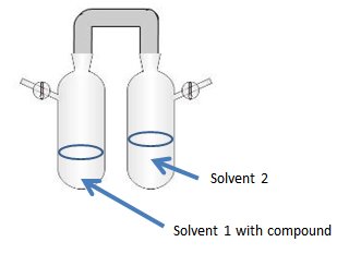
-
Layering (Solvent Diffusion): Uses the advantage of density for two different solvents. The solution (dc) is either layered under (if density of layering solvent is lighter dc > dl) or on top of (if density of layering solvent is higher dc < dl) the layering solvent (lc).
-
Sublimation: heat the sample solution under reduced pressure until it vaporizes and allow it to undergo deposition on a cool area of the surface.
Step 3: Is your molecule soluble in polar or non-polar solvents?
-
List of Polar Solvents
A. Aprotic Polar Solvents
-Acetonitrile (MeCN)
- Layer with ether, ether/hexane (1:1), acetone, acetone/hexane (1:1), dichloromethane (DCM aka methylene chloride), chloroform, toluene, THF
- Diffusion with ether, E/H, Me2CO, DCM
-Dimethylsulfoxide (DMSO)
- Layer with ether, acetone, ether/acetone
- Diffusion with E/H, Ether/Acetone, Acetone
-Dimethylformamide (DMF)
- Layer with ether, acetone, ether/acetone, hexane, ether/hexane
- Diffusion with E/H, Hexane, Ether/Acetone, Acetone
-Acetone (Me2CO)
B. Polar Protic Solvents
-Ethanol (EtOH)
- Layer with acetone, ether, ether/acetone, water, acetonitrile
- Diffuse with acetone, ether, ether/acetone
-Methanol (MeOH)
- Layer with acetone, ether, ether/acetone, water, acetonitrile
- Diffuse with acetone, ether, ether/acetone
-tertButanol (tBuOH)
- Layer with acetone, ether, ether/acetone, water, acetonitrile
- Diffuse with acetone, ether, ether/acetone
-Water (H2O)
- Layer with acetone, alcohols
- Diffuse with alcohol, methanol
-nPropanol (nPrOH)
- Layer with acetone, ether, ether/acetone, water, acetonitrile
- Diffuse with acetone, ether, ether/acetone
C. Borderline Aprotic Solvents
-Tetrahydrofuran (THF)
- Layer with alcohols, acetonitrile, DCM, nitromethane, chloroform
- Diffuse with alcohols, DCM
-Ethylacetate (Et2OAc)
-Dichloromethane (DCM)
- Layer with ether, ether/hexane, hexane, acetonitrile
D. Nonpolar Solvents
-Pentane (P)
- Layer with ether, acetone, ether/acetone, acetonitrile
- Diffusion with ether, acetone
-Hexane (H)
- Layer with ether, acetone, ether/acetone, acetonitrile
- Diffusion with ether, acetone
-Cyclohexane (CH)
- Layer with ether, acetone, ether/acetone, acetonitrile
- Diffusion with ether, acetone
-Benzene (Bz)
- Layer with ether, acetone, ether/acetone, acetonitrile
- Diffusion with ether, acetone
-Toluene (Tol)
- Layer with acetonitrile, hexanes, pentane, ether, DCM
- Diffusion with hexane, ether, DCM
-Chloroform (CHCl3)
- Layer with ether, hexane, ether/hexane, pentane, ether/pentane, acetonitrile
- Diffuse with ether, hexane
-Ethyl Ether (Et2O)
- Layer with acetone, acetonitrile, ethyl acetate, hexane
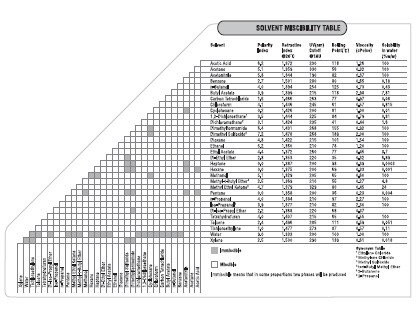
**If these solvents do not work you can also layer any solvent with another solvent it is miscible with (see chart below)
Step 4: What if crystals are not growing?
-
Try adding one of the neutral molecules to act as a cocrystallizaer.
-
Place reaction in fridge, sometimes a change in temperature (or cooler temperatures) can induct crystalliations.
-
Use a seed crystal or slightly scratch the glass to create a nucleation site.
Step 5: I have crystals but they’re not suitable for data collection. What do I do?
-
Recrystallization – dissolve your crystals in another solvent (test for solubility by using a small amount of crystals and scanning different solvents) and layer back with the solvent they originally crystallize from or one from the miscibility chart.
-
Place vial in the fridge to slow the process of crystallization and hopefully yield better crystals.
-
Decrease the concentration of your solution so the crystals have more room to form single crystals.
-
Try using a similar solvent system (i.e. chloroform for DCM, nitromethane for acetonitrile, ethanol for methanol) or a mixture of solvents (pick two solvents which are miscible).
How to Solve an X-Ray Crystal Structure with ShelXTL
Download a PDF version of this document HERE: Solving an X-Ray Crystal Structure
File
- New (give your new project a name and highlight the *.raw file)
- Open (opens an already existing project)
XPrep
- Screen shows: P A B C I ……
0.0 19.0 21.0 ……
These symbols are abbreviations for lattices (e.g. face centered, body centered, …)
You have to look for the one with the smallest value, which also determines the lattice type for your crystal. If two columns are 0 chose the one with higher symmetry.
- Select [H] and press enter and go through commands
- Before you type [F]: press [A] for absorption correction (only if crystal dimensions have been measured before data collection)
- This part of the program creates a new set of files:
- *.hkl (including the data)
- *.ins (input file for next step)
- *.prp (listing of what happened in XPrep)
XS
- Input for this program: *.ins and *.hkl
- CFOM (Combined Figures of Merit): The lower this value, the better is your collected data set (as low as 0.036)
- RE: if this value is below 10% your data is good
- The output from this program is: *.res (including the results), *.lst (listing of what happened in XS including an electron-density map)
XP
- help (gives you a list of all commands. Type help …. And receive a description of this specific command)
- info (lists all atoms and bonds of your current moiety after fmol has been applied)
- fmol (creates a list of atoms with according connectivities. If there is still fmol occurring in the prompt, just press enter until the list is complete. This command has to be applied everytime you enter XP)
- fmol/n (does the same as fmol but without showing on the screen. Later on, if you are in unique mode, by typing fmol/n you can go back to the entire molecule)
- mpln (mean least square plane: calculates the best view of the electron-density map to facilitate looking at the structure)
- mpln/n (again, no visual output)
- fmol/n $n (you will only see the nitrogen atoms)
- fmol/n rest (you will see the rest of the atoms without the nitrogens)
- proj (project: view structure: mono –> 1-dimensional; stereo –> 3-dimensional)
- eyes 1 (always view structure in 1-D)
- eyes 2 (always view structure in 3-D)
- uniq ho1 (unique: view only the specified atom here Ho1 and what it is connected to. If you then type proj you will only see Ho1 and its immediate surroundings)
- diag (like proj without a menu. If you now press enter, the picture of the structure will stay in the top right corner of your screen even if you are in prompt screen)
- kill q40 q3 (deletes specified atoms here atoms q40 and q3 irreversibly. If you now type proj, the deleted atoms will not show up any more)
- read kv01 (if you accidentally deleted an atom and you want it back, this command will re-read the *.res file until ‘END’ in the *.res file)
- reap kv01 (reads complete *.res file. After read or reap, you type fmol and proj and all the original atoms are back)
- bang q22 q1 (calculates all bond angles and bond distances for the selected atoms)
- name q22 n1 (if you are sure about the identity of a specific electron density here q22 you can name it here Nitrogen1 or n1. Note: you can’t give two separate atoms the same name)
- pick (in the window you can browse through atoms of a specific moiety and label them)
- sort (if you type sort and then info, you will see all the acquired information so far sorted by numbers)
- sort $o $n (sorts and lists all the oxygen atoms first and then all the nitrogen atoms sorted by numbers)
- file kv01 (writes new *.ins file)
- quit (exits XP)
- exit (also exits XP)
XL
- Run XL (this is the first step of the refinement. After computer is done, just press any key)
XP
- info (after fmol and mpln type info and look at the column with the Ueq values: All values for the assigned atoms should be roughly in a range between 0.02x and 0.05x.If you get 0.1xx –> you assigned too many electrons to that peak. Kill, because it is a noise peak. If you get 0.000 –> Too little electrons assigned. Take an atom with higher atomic number. If you then are missing an atom in your structure, take the q with the highest value, which should be much higher than all the others, and assign it an atom name)
- proj less $q (projects everything except q’s)
- kill $q (kill all the remaining q’s that aren’t atoms)
- file kv01
XL
- Run XL refinement cycle again
- Go back to XP and look at Ueq Make adjustments if necessary.
- Go back and forth XL and XP until all atoms and their Ueq values are okay
Edit
- copy .res –> .ins (takes the *.res file from XL and writes a new *.ins file for further steps)
- Edit .ins (opens window with the data of the *.ins file)
- Below ‘PLAN 20’ make a new line and type in a new command:
‘ANIS’ for the atoms you wish to make anisotropic
- Save and exit Editor
XL
- Run XL refinement cycle again (now XL takes sphere representation of the atoms and calculates ellipsoid representation which is more accurate)
XP
- Now you can also see some of the protons in the structure as q’s. Usually you don’t need to refine protons except Hydroxide-protons or H-bonded protons. For all the other protons you just add them later in optimized calculated positions. If you want to refine the protons, just assign q’s as protons and go back and forth between XL and XP to refine them. The Ueq values of protons are usually a little bigger than the ones for other atoms.
- kill $q
- hadd $h $c (adds protons to all unsaturated carbons. Check if all protons are in the right postion and if there is the right number of protons on all atoms. Alternatively, protons can be added in the *.ins file. Under ‘PLAN 20’ write ‘HFIX 137 c1 c2’ to add protons to c1 and c2)
- atyp 2 5 $c (set colors and style of all carbon atoms. First number encodes the type, second number encodes the color of the chosen atoms. Type help atyp to see a list of all the colors and styles)
- file kv01 (writes new *.ins file with anisotropic refinement)
XL
- Run another XL refinement cycle
Edit
- Edit .ins
- See ‘Afix 43’ (different for every atom. First number tells you the hybridization of the atom. 4 is aromatic carbon, 3 is methyl carbon, 2 is methylene carbon)
- See ‘Afix 0’ (terminates the project for one atom and moves on to the next)
- copy .res –> .ins
- Edit .ins
- Below ‘TEMP -100’ make a new line and type in a new command:
‘OMIT -3 55’ (this tells XL to only use reflections within 2 θ = 55o)
- Save and exit Editor
XL
- Run another XL refinement cycle (Before you exit XL look at the WR2 and R1 value)
Advanced Refinement
- Atoms that are not behaving properly—modify in the .ins file:
- Atom moving too much
- DFIX:
- The distance between the first and second named atom, the third and fourth, fifth and sixth etc. (if present) is restrained to a target value d with an estimated standard deviation s.
- Use DFIX 1.54 0.01 A B, where 1.54 is the distance, 0.01 is the standard deviation, A is the first atom, B is the second atom
- SADI
- The distances between the first and second named atoms, the third and fourth, fifth and sixth etc. (if present) are restrained to be equal with an effective standard deviation s.
- SADI 0.02 A B, 0.02 is the standard deviation, A is the first atom, B is the second atom
- SAME
- The list of atoms (which may include the symbol ‘>’ meaning all intervening non-hydrogen atoms in a forward direction, or ‘<‘ meaning all intervening non-hydrogen atoms in a backward direction) is compared with the same number of atoms which follow the SAME instruction.
- Use for a set of atoms: SAME C1> C6 before C11 > C16, where C1 … C6 is an ideal benzoate and C11 > C16 is an unideal benzoate. Also good for t-butyl group
- Displacement parameters are too high or too low
- EADP
- The same isotropic or anisotropic displacement parameters are used for all the named atoms. The displacement parameters (and possibly free variable references) are taken from the first atom in the atom list that is linked to other atoms by EADP.
- Use this command for methyl groups in tert-butyl groups, F– ions in PF6–
- RIGU
- Apply enhanced rigid bond restraints with esds s1 for 1,2-distances and s2 for 1,3 [Thorn, Dittrich & Sheldrick,Acta Cryst. A68 (2012) 448-451].
- Use RIGU for all atoms
- EADP
- DFIX:
- Atom moving too much
Modeling disorder
- Use parts with defined occupation factor
- PART 1 10.6 C1 > C6 PART 2 10.4 C1’ > C6’
- Where 10.6 is the occupation factor of part 1, 10.4 is the occupation factor of part 2, C1 > C6 are the main atoms, C1’ > C6’ are the disordered atoms
- Use parts and use a free variable
- PART 21 C1 > C6 PART 0
- PART -21 C1’ > C6’ PART 0
- FVAR line 0.08 0.6
- 21 defines part1, -21 defines part2, PART 0 end the command line so only a set list of atoms are included in the disorder
- 0.08 is the free variable for all atoms (already in the .ins) 0.60 is the 2nd Free variable linked to 21. To use further parts just add further lines (i.e. part 31 part -31 part 41 part -41, FVAR 0.08 0.60 (#fvar3) (#fvar4)
- Adding hydrogen atoms to non-carbon atoms (modify in XP)
- Use HADD:
- HADD 8 O1 (adds 1 hydrogen atom to O1, making it a hydroxide)*
- HADD 9 O1 (add 2 hydrogen atoms to O1, making it a water)*
- HADD 4 C4 (add one proton to C4 because it is aromatic, can be used if hadd $c does not add correct number of hydrogens)
- For more information on hydrogen codes type HELP HADD
- Use HADD:
**applicable for either group (i.e. N, C, etc.)
Edit
- copy .res –> .ins
- Edit .ins
- Go down (all the way to the bottom) and look for a line with: ‘WGHT …’
- Copy this line
- Go back up and look for another line with ‘WGHT …’ under ‘PLAN 20’
- Overwrite this line with the other line from the bottom (This tells XL to use a weighting-scheme of the reflections including errors which is proposed by the computer)
- Save and exit Editor
XL
- Run another XL refinement cycle (Now WR2 and R1 value should have gone down)
- Go back into *.ins file, copy the ‘WGHT …’ line again, run XL again… Go back and forth until WR2 value doesn’t change significantly any more)
XP
- kill $q
- info less $h (you can see that the labels are not in order)
- pick (rename all the atoms in an orderly fashion)
- sort (now atoms are sorted in info-list)
- sort $cl $n (sort in order of atomic numbers)
- hadd $c (H’s are placed after the carbon they are attached to)
- save kv02 (Saves this session. Take a name different from the overall project name. This is a good point the save because all the atoms are labeled, refined, …)
- next kv02 (To continue where you left from with the save command)
- fmol (creates a list of atoms with according connectivities. If there is still fmol occurring in the prompt, just press enter until the list is complete)
- file kv01
Edit
- Edit .ins
- Below ‘L.S. 4’ make two new lines and type in the new commands:
‘ACTA’ and
‘BOND $H’
- Save and exit Editor
XL
- Run another XL refinement cycle (now XL creates a new set of files: *.cif crystallographic information file and *.fcf)
Edit
- copy .res –> .ins
- Below ‘PLAN 20’ make a new line and type in a new command:
‘CONF’ (this adds a list of torsion angles to the *.ins file)
- Save and exit Editor
XL
- Run another XL refinement cycle
XP Codes
- envi $cl (calculates environment around specified atom)
- envi $cl 1.5 (gives environment around specified atom but with higher tolerance. You can see a larger number of atomic interactions. With this tool you can see if there are any interactions of the specified atom to any atoms that are not directly bonded to it. If an interaction is present, that atom will have a symmetry label different from 1555)
- symm (tells you what symmetry you have. The 555 represents the asymmetric unit. Example: 1555: first 5 is x- coordinate, second 5 is y, third 5 is z. 1 is symmetry operation. 1655 is a translation in the x-direction. 1565 is a translation in the y-direction. A 2 means inversion, which you can also see with the presence of –x, -y and –z)
- proj cell (see the molecule and the unit cell)
- sgen 2666 (generates a symmetry-equivalent molecule. Here: inversion (2) followed by a translation in all directions (666) result: 1-x, 1-y, 1-z)
- fuse (fuses all the symmetry-equivalent molecules back to one molecule. By typing fuse cl1 cl1a you can fuse atoms that are symmetry-equivalent)
- envi $cl (here: see that one Cl has interaction with another molecule symm. Create second molecule with sgen 2775 and see interaction)
- link cu1 cl1a (creates a dashed bond between specified atoms of the two interacting molecules)
- undo c1 c7 (kills the bond between specified atoms)
- link1 cu1 cl1 (makes a dashed bond solid, if you accidentally made a real bond dashed)
- prun cu1 (removes all the bonds from the specified atom)
- matr1 (makes a-axis perpendicular to the screen in a projection. matr2 makes b-axis perpendicular, …)
- matr 1 1 1 (makes the diagonal of the unit cell perpendicular to the screen)
- ↑ (up-arrow on keyboard brings back old commands)
- cell (displays unit cell parameters. Put shortest axis perpendicular to screen with matr command)
- pack (packs molecules in unit cell. Dashed lines represent intermolecular interactions. ‘Scan Mols.’ unit cell blinks (like pick command). ‘scan non-B’ scans dashed lines and delete what you don’t need or want. ‘sgen/fmol’ displays what you constructed in packing diagram.)
- info (all those symmetry operations added new labels to the atoms)
- name ???a ???(renames atoms that had an XXXA label back to XXX)
- mpln (gives the best plane with deviations of atoms from that plane)
- nopl (undoes all mpln commands and deletes all previous planes)
- mpln n1 c1 … (creates best plane including specified atoms)
- mpln n2 c6 … (creates this plane and shows you the dihedral angle between this plane and the previous plane. The numbers on the left side of an atoms show how far the atom is away from the plane. Good way to check the planarity of a ring. If numbers are really small you know that the specified atoms are in plane)
- telp 0 -50 0.025
(telp creates a drawing of the molecule. In the drawing, put labels next to atoms. First number encodes type of drawing, second number is %age of thermal ellipsoids, and third number is thickness of the bonds. After you are done, press ‘Esc’ or ‘h’ to exit without saving, press ‘Enter’ or ‘b’ to exit with saving)
- exam *.plt (exam works like a directory command and shows you a list of all files with .plt extension)
- labl 1 400 (determines which atoms get labeled and in what style they get labeled)
- link 5 $h (makes all bonds to hydrogen atoms a line to distinguish them from other bonds)
- view drawing1 (to see the drawing on screen)
- draw drawing1(chose ‘h’ for hpgl-file and then go through commands. Now you can insert this *.hpgl file into word and see it as a picture)
- cent n1 c1… (calculates the center of the specified ring)
- cent/x n1 c1… (calculates the center of the specified ring and puts an imaginary atom in that position. If you need to calculate the distance between two rings, this is a good method)
Edit
- Since XP can’t calculate the error of a value (which you need in publications), you have to do this in the *.ins file
- Below ‘PLAN’ make a new line and type in a new command:
‘MPLA 6 n1 c1 > c6 cu’ (this will calculate the ring n1 through c6 and will then calculate the distance of Cu to that specific ring. The 6 means that the first 6 atoms are included in the ring calculation but not Cu. You can use this to determine if for example a given molecule is square planar or not)
- Save and exit Editor, run XL refinement cycle and see the result in *.lst file
- Below ‘PLAN 20’ make a new line and type in a new command:
‘EQIV $1 1-x 1-y -z’ (this will define a certain symmetry operation and give it the name $1)
- Then type:
‘RTAB ang1 cl2_$1 cu1 n1’ (calculate the angle between the specified atoms linked through the specified symmetry operation)
- Below ‘PLAN 20’ make a new line and type in a new command:
‘HTAB’ (htab is for calculating Hydrogen-bonds if present. You can see the hydrogen bonds in the *.lst file)
- If your hydrogen bond is within the same symmetry unit, add the following under the ‘HTAB’:
‘HTAB o1 n2’ (calculates the H-bond between o1-H….n2)
- If your hydrogen bond is in a different symmetry unit, you have the specify the symmetry operation first (which can be found in the *.lst file behind that specific H-bond) by typing:
‘EQIV $1 x-1, y, z+1’ (You can just copy and paste the symmetry operation from the *.lst file. $1 is now the name of that specific symmetry operation)
- Now add:
‘HTAB o1 n2_$1’ (calculates the specified H-bond between o1-H….n2 with n2 being from a symmetry related molecule)
Finalizing a project
Modify *.cif
- Open modify.cif
- Open *.cif
- Replace the specified line with those from the modify.cif file
- The ‘number of reflection used’ can be found in the *.p4p file
- Save *.cif
XCIF
- Table of choices:
- Chose [R] then enter name of *.ref file, enter (reference file)
- [y] enter
- select modified *.cif file, enter
- name of file needs to be modified enter
- Chose [C] here you can set the compound name (usually you don’t change the name, because it has been assigned correctly at data collection)
- Chose [T] here you create all the necessary tables
- take *.cif file, enter
- [y] enter
- filename: here, type: *.rtf
- filename extension: rtf
(don’t add ‘hydrogen atom coordinates table’,’torsion angles table’ and ‘hydrogen bond table’ unless you specifically want them)
- [F]: tabulation of intensity data (usually not required)
- Chose [Q] enter (to quit the program)
Edit *.rtf file / Write *.tbl.docx
- Open the *.rtf file
- Run the ‘tbl’ macro
- Save document as *.tbl.doc
Write *.exp.doc
- Open the generic experimental file
- Replace the bold values with the real values for your compound
- Unbold the numbers
- Save document as *.exp.doc
XShell
- Open your project
- Kill the q’s
- Save file as *.pdb (If you have to create a symmetry equivalent, chose ‘save all’ command)
Drawings
- Make one black and white and one colored drawing of the molecule in XP
- Insert the drawings into a word document and save it as *.drw.docx
- Link 5 $h
- Labl 1 400
- Telp 0 -50 0.025
Send Project Back
- Go to x-ray management site
- Chose submission editor
- Enter project code and search
- When project is found, click on the project number to open project
- Go to ‘Status’ and change it to ‘Write Experimental’
- Go to ‘Assigned to’ and change it to ‘Khalil Abboud’
Adding a project to the database
Create Files
- Go to the project folder on the X-drive
- Create a new folder inside the project folder with the project name
- Copy important files into this new folder:
- *.cif
- *.tbl.docx
- *.exp.docx
- *.drw.docx
- *.fcf
- *.pdb
- *.res
- Create a *.zip file from this folder
- Move files to the ‘Final Projects to be added’ folder: *.pdb, *.zip, Entire project folder
Database
- Open the ‘Final Projects to be added’ folder
- Open the ‘X-ray secure data’ folder
- Add the *.pdb file under the professors name (change security variables)
- Add the *.zip file into the download folder (change security variables)
- Add the *.zip file to ‘Archived Projects’ folder under ‘Zipped’
- Add the entire project folder to ‘Archived Projects’ folder under ‘Unzipped’
Update Database
- Go to x-ray management site
- Chose submission editor
- Enter project code and search
- When project is found, select the ‘Update Database’ button
- In the next window, browse for the *.cif on the X-drive, open it and press ‘go’
- Email student
Finish
- Go to x-ray management site
- Chose submission editor
- Enter project code and search
- When project is found, click on the project number to open project
- Go to ‘Status’ and change it to ‘Done’
- Go to ‘Assigned to’ and change it to ‘Not assigned’
- Click the ‘Generate Invoice’ button
- Click on ‘email’ to send an email to the business office and confirm
How to Apply Absorption Correction to X-Ray Data
Download a PDF version of this document HERE: Applying Absorption Correction
After solving structure, tending to disorder, solvents, etc.:
This details absorption correction applied according to indexed faces. The process requires a correct molecular formula.
- Open XP
- Kill $H, note number
- Kill $C, note number
- so you know total molecular formula that you expect in unit cell
- Does this include solvent?
- Make note of the chemical formula (ex: C20 H24 N2 O3 Mn3 etc.)
- Open cmd.exe
- Set directory to X: (or current working directory)
- Cd 1415 (or current fiscal year folder)
- Cd project name
- Open file mo_name_0m.p4p and edit in the chemical formula on the line:
- CHEM ?
- By replacing the ? with the actual formula you noted above
- Cmd: xprep mo_name_0m.raw
- Find symmetry/space group, make sure it matches what you solved
- Go through statistics
- Find formula/content of unit cell
- Select [A] for absorption correction
- Select [F] to correct based on faces
- Psi scans if no faces
- Check faces
- Wavelength
- Current absorption coefficient
- Name of file with directional cosines should be i.e. mo_name_0m.raw
- Copy whole of input file with updated I and sigma? Say Yes instead
- Output file name *.abc
- [E] exit to xprep menu
- [F] to create shelxtl files
- Output file name face
- Format [s]
- Write face.* files
- Select [F] to correct based on faces
- Open face.ins, solved structure .ins
- Copy from OMIT to just before HKLF from *.ins
- Paste to replace TREF in face.ins
- Back to CMD: xl face (no extension)
- Check R1, wR2,GooF values
- R1 after merging, highest peak, deepest hole
This process details absorption correction using the program SADABS. Absorption of this type is known as correction by “psi-scans”.
- Run SADABS
- [N] no expert mode
- Select Laue mode (should be space group minus translational symmetry…)
- Enter file name of data (mo_name_0m NO EXTENSION)
- Go through defaults
- It will go through 25 cycles
- Look at wR2 for 1-25 to make sure it decreases
- Accept [A]
- SADABS part 2: defaults
- SADABS part 3
- Write postscript [Y], sad.eps, enter through [test]
- [W] write hkl
- hkl
- Quit SADABS [Q]
- Copy *.p4p p4p
- XPREP abc
- Edit abc.ins with OMIT through HKLF for TREF
- XL abc
- Cycle WGHT (full line) and refine
- Copy bottom WGHT value to top in .res
- Copy .res -> .ins
- Xl
- Watch GooF values and wR2 values (should decrease)
It is important to apply the type of correction that makes the most sense for your crystal. For example, a crystal that does not contain heavier atoms, like transition metals, is typically not treated using correction by faces.
The final .cif file should be amended to include comments about the type of correction applied, if any.
ABSORPTION OPTIONS
_exptl_absorpt_correction_type
#explanation: analytical from crystal shape
face.* analytical
_exptl_absorpt_process_details
‘based on measured indexed crystal faces, Bruker SHELXTL2014 (Sheldrick, 2014)’
#explanation: empirical from intensities
abc.* empirical
_exptl_absorpt_process_details
‘SADABS, Blessing, R.H. (1995). Acta Cryst. A51, 33-38.’
#explanation: numerical from crystal shape
hkl.* numerical
_exptl_absorpt_process_details
‘based on measured indexed crystal faces, Bruker APEX2 (Bruker, 2014)’
#explanation: psi-scan corrections
psi.* multi-scan
#explanation: no absorption correction applied
none